|
|
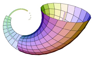
To describe our central image in technical language, we have to define a central curve X(t) over a parameter t. The curve we chose is an arithmetic spiral lifted onto a cone, with equation
X(t) = (tcos(t), tsin(t), pt). The radius function r(t) that describes the expanding cone is given by 0.8e0.6t.
- As t goes from 0 to p/2, we show a number of points on the curve. From p/2 to p, we show the curve itself, actually represented by a thin tube.
- From p to 3p/2, we show a "normal strip" of the form
X(t) + rP(t) where r goes from -r(t) to r(t). Here P(t) corresponds to the principal normal, a unit vector perpendicular to T(t), the unit tangent vector of the curve and lying in the plane determined by the velocity and the acceleration of the curve.
- From 3p/2 to 2p, the figure is an expanding cone, or "cornucopia". The equation of the circular slice for each t is
X(t) + r(t)(cos(u)P(t) + sin(u)B(t)) where B(t) is the unit binormal vector perpendicular to T(t) and P(t), and where u is a parameter that goes from 0 to 2p.
Thus the image grows not only in size, but but also in dimension.
If we continue to the next section of the curve, from 2p to 5p/2, the slices will be two-dimensional spheres, given by
X(t) = r(t)(cos(v)cos(u)P(t) + cos(v)sin(u)B(t) + sin(v)W(t)) where W(t) is a unit vector in 4-space perpendicular to T(t), P(t), and B(t). We can project this slice into our 3-space by pushing W(t) down to T(t), and this is the view we show on the previous page.
|
|