Bernhard Riemann, a student of Gauss, saw how to explore the geometry of a two-dimensional surface without having to know the way it was situated in space. He realized that if it was possible to calculate the length of a curve on the surface, then he could also figure out the area of any region on the surface, and he could determine how "curved" a curve was at a point by measuring its deviation from "straightness".
In order to make these ideas precise, it is necessary to use some ideas from calculus of one variable, and then to generalize them further. The formula for arclength of the graph y = f(x) of a function of the variable x over the interval from a to b is given in most textbooks as an application of integration. By approximating the graph by polygons with shorter and shorter sides we find Riemann sums that approximate the length, and in the limit we obtain
L = ∫ab&radic(1 + f'(x)2)dx
A similar process leads to the formula for the area of a surface of revolution of the function graph about the x-axis, yielding
A = ∫abπf(x)√(1 + f'(x)2)dx
We can apply these formulas to the surfaces of revolution most important for the study of non-Euclidean geometry, namely the sphere and the pseudospherical surface introduced in Chapter 10. The sphere of radius R is given by the surface of revolution of
L = R∫-RR(1/√(R2 - x2))dx
= R[sin-1(x/R)]-RR
= πR
The integrand for the area is even simpler,
A = ∫abπRdx = (b-a)πR
It is difficult to find an explicit function for the tractrix mentioned in Chapter 10, and it is easier to work with curves given in parametric form. For a curve (x(t),y(t)) given by two differentiable coordinate functions x(t) and y(t), the velocity vector to the curve is given by (x'(t),y'(t)) and the length of the velocity vector gives the speed of the curve, denoted
The pseudosphere can be described as the surface of revolution of the curve
y'(t) = cos(t), so
s'(t) = √(1/sin2(t) - 1) = cot(t)
The length of the curve is then
L = ∫abcos(t)dt = [ln(sin(t))]a b
The area will be
It follows that the area of the pseudosphere is finite.
An application of integration found in many calculus textbooks is curvature of curves. The definition of curvature for a curve in the plane is the derivative with respect to arclength of the angle that the tangent line makes with the horizontal axis. For a function graph y = f(x) we obtain
κ(x) = θ'(x)/s'(x) = f''(x)/(1 + f'(x))3/2
For the curve
For a parametric curve (x(t),y(t)), if x'(t) ≠ 0, the angle is given by
θ(t) = tan-1(y'(t)/x'(t))/s'(t) = (y''(t)x'(t)-y'(t)x''(t))/(x'(t)2 + y'(t)2)3/2.
For the circle of radius R,
For the tractrix,
We have s'(t) = cot(t) and curvature
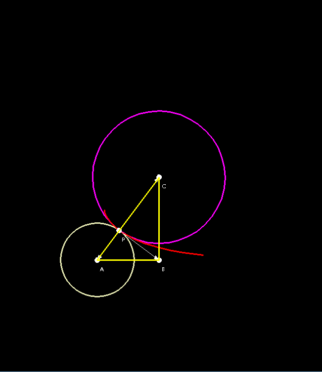
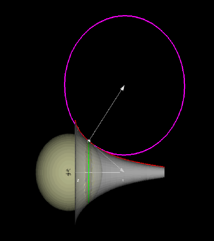
Euler proposed a measure of curvature of a surface of revolution at a point as the product of the curvature of the profile curve at the point and the length of the projection of the curvature vector of the circle through the point to the normal line at the point. This second curvature is given by the formula
Demonstration
Gauss discovered another way of dealing with the geometry of surfaces, using techniques from multivariable calculus. He reasoned that if a surface in ordinary three-space was given by a vector equation X(u,v) with partial derivatives Xu(u,v) and Xv(u,v), then for any curve (u(t),v(t)) in the domain, the velocity vector of the curve X(t) = X(u(t),v(t)) is given by the chain rule:
The square of the arclength is
abbreviated ds2 = Edu2 + 2Fdudv + Gdv2. Once we know these three functions E(u,v), F(u,v), and G(u,v), over the domain, we can compute the length of any curve on the surface defined by a curve in the domain, even if we are not given the equation of the surface.
As an example, the sphere of radius R in geographical latitude-longitude coordinates is given by X(u,v) = (Rcos(u)cos(v),Rsin(u)cos(v),Rsin(v)) with partial derivatives
Xv(u,v) = (-Rcos(u)sin(v),-Rsin(u)sin(v),Rcos(v)).
Thus E(u,v) = R2cos2(v), F(u,v) = 0, and G(u,v) = R2.
For a surface X(u,v), the area of a domain is given by the integral of the length of the cross product Xu(u,v) x Xv(u,v), so the area is
But
It follows that if we know E, F, and G, we can determine the area of any region on the surface by integrating √(EG - F2) over the domain.
For a region on the sphere determined by a ≤ u ≤ b, c
≤ v ≤ d, we can find the area by integrating √(EG - F2) =
R2cos(v) over the region to get Area = R2(b - a)(sin(d) - sin(a)).
The truly amazing thing is that we can now compute lengths and
areas for curves and regions on the plane once we are given the "metric
coefficients" E, F, and G. One of the most important examples is the case
where the domain is the upper half plane
Consider the functions E(x,y) = 1/y2 = G(x,y) and F(x,y) = 0. Then the length of a curve (x(t),y(t)) is the integral of s'(t)2 = E(x(t),y(t))x'(t)2 + 2F(x(t),y(t))x'(t)y'(t) + G(x(t),y(t))y'(t)2 = (1/y(t)2)(x'(t)2 + y'(t)2). For example, if x(t) = t, and y = c for t going from a to b, the length is
Note that the distance between two parallel vertical lines x = a and x = b becomes smaller and smaller as the y-coordinate c increases. For a vertical line, if x(t) = a, a constant, and if y(t) = t for t going from c to d, the length is the integral of (1/t) from c to d, namely ln(d) - ln(c). As d increases, the length of this segment goes to infinity.
The area of the region where x goes from a to b and y goes from c to d in this metric will be
Note that as d → ∞, this area is bounded by (b-a)/c.
We can try to find the shortest curve from (a,c) to (a,d), and we can show that we already have it. We have to integrate 1/y(t)√(x'(t)2 + y'(t)2) ≥ |y'(t)|/y(t)| from t = t0 to t1, where y(t0) = c and y(t1) = d. The most efficient paths will have x'(t) = 0, so x(t) = a for all t, and y'(t) > 0 so the integral is
Thus the vertical lines in this metric on the upper half plane are geodesics, representing the shortest curves from one point to another on the same vertical line.
For points not on the same vertical line, it is somewhat harder to
determine the shortest curve joining the points by a curve in the upper
half plane, measured in this strange metric. This process is simplified
considerably by the results we have already obtained in Chapter 10, since
it turns out that the linear fractional transformations on the upper half
plane preserve the lengths of curves. As in Chapter 10, we write the
curve using complex numbers z = x + iy. so the curve is given by
For a linear fractional transformation w = (Az+B)/(Cz+D) for real numbers A, B, C, and D with AD-BC = 1, we already know that
and we compute
Thus the arclength of the curve w(t) is the same as the arclength of the curve z(t). We say that the linear fractional transformations are "isometries of the upper half plane with the hyperbolic metric".
We have already shown that it is possible to send a vertical line to a circle with center on the x-axis by a linear fractional transformation. This makes it possible to compute the distance between two points in the upper half plane using this metric. First we find a circle with center on the x-axis passing through the two points. We then find a linear fractional transformation taking one of the points to the point i with coordinates (0,1) and the other to a point on the vertical axis (0,M) with M > 1. Since the distance from i to Mi is ln(M), and since the linear fractional transformation is an isometry, it follows that the distance between the original two points is ln(M).
In particular it follows that the arcs of circles centered on the x-axis represent the shortest paths between any two points on the arc, These semicircles and the vertical lines represent the geodesics in this geometry. In this way, we have shown how the way of measuring described by Gauss enables us to define a geometry by means of metric coefficients.
Gauss in his original treatises on surfaces proved some remarkable theorems concerning curvature of surfaces. He defined a function Κ(u,v) on a surface that generalizes Euler's construction for surfaces of revolution, and he showed that this function could be computed just using the metric coefficients E, F, and G. He was so impressed by this result that he named it the "Theorema Egregium". In the case of the upper half plane with the hyperbolic metric, the curvature turns out to be constantly equal to -1.
Even more remarkable is a theorem relating the area of a triangle to the sum of its interior angles. We have already shown that the area of a strip bounded by two vertical lines and a vertical segment is bounded. It is also true that the area above the arc of a circle with center on the x-axis and between two vertical strips meeting the circle will be bounded, and in fact it will be π - (sum of the angles). Once we have this fact, we can show that the area of any triangle will be π the sum of the three angles.
This result is part of a much more general result proved in
courses in differential geometry, namely that for a triangle with geodesic
sides, the integral of the Gaussian curvature Κ equals 2π - ∑ext.angles. For the ordinary Euclidean plane with Κ = 0, this just
states the familiar theorem that π = sum of interior angles. On a unit
sphere, with