|
Linear Functions
Text Calculus is the study of functions.
 In the study of functions of
one variable, we encounter domains and ranges of functions, function
graphs, and properties of functions such as continuity. In multivariable
calculus we will extend all of these notions to functions of two and
eventually more variables. We will also deal with functions of one
variable associated with functions of a single variable, namely slice
curves and contour lines.
In the study of functions of
one variable, we encounter domains and ranges of functions, function
graphs, and properties of functions such as continuity. In multivariable
calculus we will extend all of these notions to functions of two and
eventually more variables. We will also deal with functions of one
variable associated with functions of a single variable, namely slice
curves and contour lines.

Demos
Linear Functions
| 
|
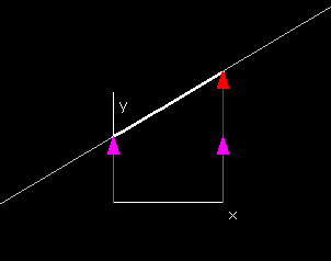
This demo shows the linear function in one variables L(x) = px +k over the domain 0 ≤ x ≤ 1. You can change the constants p and k using the respective red or purple slide bar, and the Graph: L(x,y) window will show the function graph of L(x,y) with the chosen values for the constants.
If you slide the hotspot on the purple slidebar, (thereby varying the constant k) the function graph is translated up and down in the directon of f(x,y,z). Varying p on the red slidebar will scale in the x-direction of the graph.
Note: For help on using demos, see page 1 of lab 2.1.1.
|
Examples Zero Functions
The simplest function of all is the zero function,
defined by f(x) = 0 for all x. This function can be defined for any domain, and the range will
always always be the single point { 0 }.
Constant Functions
The next simplest class of functions are the constant functions
defined by f(x) = k for all x. A constant function can be defined for any domain, and the range will always always be the single point { k }.
Linear Functions
Linear functions are the next most complicated class of functions, defined
by L(x) = px + k. The number p is called the slope of the linear function and k is called its y-intercept. The natural domain of the linear function is all real numbers x. If p ≠ 0, then the range of L is all real numbers.
Exercises 1. Find the segment joining the x- and y-intercepts for y = px + k. Describe the segment.
2. Show that if p ≠ 0, then for every y there is a point x such that L(x) = px + k = y.
|