Multivariable Calculus

Directional Derivative 3D Contents

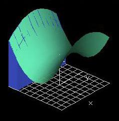
Consider a point P = (x₀,y₀) in the domain of f(x,y). The line in the domain corresponding to the direction θ will have the parametric form (x₀ + t cos θ, y₀ + t sin θ) and the height function z(t) associated with the slice curve along this line will have the form z(t) = f(x₀ + t cos θ, y₀ + t sin θ).

The directional derivative ∇_θf(x₀,y₀) at the point P will be the derivative of z(t) evaluated at t = 0 ∇_θf(x₀,y₀) = z'(0) = ∂/∂t (f(x₀+t*cos(θ),y₀+t*sin(θ)))|_t
=
0.

Note that the partial derivatives f_x and f_y are just the directional derivatives at θ = 0 and θ = π/2, respectively.

Also note that the directional derivative is a function of the direction variable θ; the variable t is only used as a parameter.

[D]

Exercises

Find the value of θ for the maximum directional derivative of any slice curve. What θ gives the minimum directional derivative for this same slice curve? How are these values related? Try this for several different slice curves.

Second Partial Derivatives 1D 3D Polar Coordinates Parametric Equations Top of Page Contents

A second partial derivative is a partial derivative of a function which is itself a partial derivative of another function.

For example, one could take the partial derivative of some function f(x,y) with respect to x, and then take the partial derivative of the resulting function f_x(x,y) with respect to y, generating the function f_yx(x,y).

There are four types of second partial derivatives:

1. f_xx(x,y) = Partial derivative of f_x(x,y) with respect to x.

2. f_yx(x,y) = Partial derivative of f_x(x,y) with respect to y.

3. f_xy(x,y) = Partial derivative of f_y(x,y) with respect to x.

4. f_yy(x,y) = Partial derivative of f_y(x,y) with respect to y.

Third, fourth, fifth, and in general, nth partial derivatives for any positive integer n, exist as well.

This is because the progression from first to second partial derivatives can be continued in the same way indefinitely. For example, to get f_xyxy(x,y), take the partial derivative of f_xy(x,y) with respect to y, and then take the partial derivative of the result with respect to x.

[D]

[D]

Exercises

1. Try entering each of these expressions for f(x,y). Note how the graphs of the second partial derivatives relate to the curvature of the graph of f(x,y):

0
1
Any constant
x
x²/2
y
y²/2
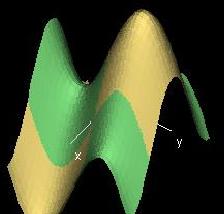
x²-y² (saddle)
x² - y⁴+y² (twin peaks)
xy
x²/2+y²/2+xy
x²*y²

2. For polynomial functions of two variables, what are the conditions needed to yield a nonzero value for each of the following?

f_xx(x,y)
f_yy(x,y)
f_xy(x,y)
f_yx(x,y)

3. a. For each of the functions in part (1), what can you say about the relationship between the mixed partials (f_xy(x,y) and f_yx(x,y))?

b. Now enter the function f(x,y) = 4xy * (x² - y²)/(x² + y²) in the second demo. Look at the curves on the first partial derivative graphs which display the second derivatives. Are any of the second partial derivatives defined at (x,y) = (0,0)? How does this differ from your observations in part (a)? (This is discussed further in the lab on equality of mixed partials.)

Hessian Determinant 1D Top of Page Contents
(Corresponds to Convexity/Concavity in 1D)

The Hessian determinant of a function f(x,y) is defined as H(x,y) = f_xx(x,y)f_yy(x,y) - f_xy(x,y)f_yx(x,y).

The Second Partials Test states that if a function f(x,y) has continuous second partials and f_x(x₀,y₀) = 0 and f_y(x₀,y₀) = 0, then

1. H > 0 and f_xx(x₀,y₀) > 0 implies (x₀,y₀) is a local minimum;

2. H > 0 and f_xx(x₀,y₀) < 0 implies (x₀,y₀) is a local maximum;

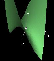
3. H < 0 implies (x₀,y₀) is a saddle point;

4. H = 0 then the test is inconclusive.

[D]

[D]

Exercises

1. For each of the following functions, find the sign of the Hessian determinant at (x,y) = (0,0) as a function of c. Verify your results using the demo.

f(x,y) = x² + cy²
f(x,y) = x² + cxy
f(x,y) = sin(x) + c cos(y)

2. Is it possible to have a surface with two or more distinct "saddles" and no "bowls"? Why or why not?

3. How could you describe a mountain range using Hessian determinants?

Taylor Series 1D 3D Top of Page Contents

Taylor Series are polynomials that approximate functions.

For functions of two variables, Taylor series depend on first, second, etc. partial derivatives at some point (x₀, y₀).

Let P₁(x,y) represent the first-order Taylor approximation for a function of two variables f(x,y). The equation for the first-order approximation is P₁(x,y) = f(x₀,y₀) + (x - x₀)f_x(x₀,y₀) + (y - y₀)f_y(x₀,y₀). We are already quite familiar with this equation since it defines a tangent plane.

Let P₂(x, y) represent the second-order Taylor approximation. Its equation is P₂(x,y) = f(x₀,y₀) + (x - x₀)f_x(x₀,y₀) + (y - y₀)f_y(x₀,y₀) + 1/2(x - x₀)²f_xx(x₀,y₀) + (x - x₀)(y - y₀)f_xy(x₀,y₀) + 1/2(y - y₀)²f_yy(x₀,y₀). To simplify, we can subsitute g(x,y) (the first order Taylor approximation) for the first three terms:

P₂(x,y) = P₁(x,y) + 1/2(x - x₀)²f_xx(x₀,y₀) + (x - x₀)(y - y₀)f_xy(x₀,y₀) + 1/2(y - y₀)²f_yy(x₀,y₀)

In general, the nth order taylor approximation for a function f(x, y) is the polynomial that has the same nth and lower partial derivatives as the function f(x, y) at the point (x₀, y₀).

[D]

Exercises

1. Try entering for f(x,y) several polynomial functions of degree less than 3. What do you notice?

2. Now enter for f(x,y) any polynomial function whose x terms have degree less than 3 but whose y terms may have degrees of 3 or greater. (For terms involving both x and y, the exponent of x should never exceed 2. e.g.: x²y³ is an acceptable term.) For example, try the function f(x,y) = y⁴ + xy² + x² + x + y. Compare the results to those of exercise 1.

3. Enter the expression 1/(x + 1) + 1/(y + 1) for f(x,y). Notice that the tangent paraboloid is not the same as the function graph. Why can't we apply the degree less than 3 rule here?

Constrained Maxima and Minima 1D 3D Polar Coordinates Parametric Equations Top of Page Contents

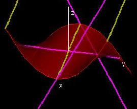
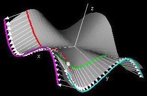
A special case of the chain rule occurs when z(t) = f(x(t),y(t)) = c is constant.

In that case, (x(t),y(t),c) is called a level curve of the function and (x(t),y(t)) is called a contour of the surface.

We then have

0 = c' = z'(t) = f_x(x(t),y(t))x'(t) + f_y(x(t),y(t))y'(t) = ∇f(x(t),y(t))⋅(x'(t),y'(t)).

It follows that the gradient of a function of two variables at a point (x(t),y(t)) is perpendicular to the tangent vector to a level curve through the point.

If the gradient at a point is not the zero vector, then all tangent lines to level curves through the point will be parallel. This follows since the intersection of the horizontal plane (x,y,c) and the non-horizontal normal plane will be a single line and all tangent lines to level curves at the point must lie in this intersection.

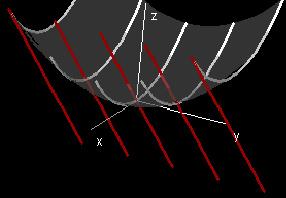
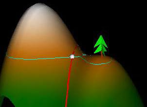
The highest point on the Massachusetts Turnpike is indicated by a sign somewhere in the hilly region of Western Massachusetts. This point will occur when the gradient vector of the turnpike's path is either the zero vector or when it is perpendicular to the turnpike's tangent vector. In the first case, the turnpike's maximum height occurs at a critical point of the surface of Western Massachuetts. In the second case, the turnpike's maximum height occurs when it is tangent to a contour line.

[D]

Exercises

1. Use the double arrow button for the variable c to determine the highway's highest point. How are the path's tangent vector (light grey) and the surfaces gradient vector (yellow) related, as seen in the "Domain" window? At what angle is the gradient slice curve (yellow) cutting the curve (red) on the surface, as seen in the "Scenic Highway" window?

2. Try entering w(t)=(t,t) and determine the highest point on the highway for this new path. What happens to the gradient vector (yellow) at the highest point? What happens to the gradient vector on either side of the highest point? What kind of critical point is this? Why?

The Gradient Vector Field Top of Page Contents

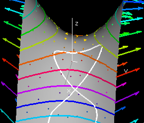
The gradient vector of the function f(x,y) at a point (x,y) is defined as gradf(x,y) = (f_x(x,y),f_y(x,y)).

By the chain rule, if (x(t),y(t)) is a parametrized curve in the plane, then the derivative of z(t) = f(x(t),y(t)) is z'(t) = f_x(x(t),y(t))x'(t) + f_y(x(t),y(t))'(t) = ∇f(x(t),y(t))*(x'(t),y'(t)). Thus at a maximum or minimum value of z(t) on the curve, the gradient vector of the function is perpendicular to the tangent vector of the curve. In particular if the curve is a contour of the function, so that z(t) is constant, then the gradient vector is perpendicular to the contour at all points.

[D]

Equality of Mixed Partials Polar Coordinates Top of Page Contents

If f(x, y) is a twice continuously differentiable function then f_xy(x, y) = f_yx(x, y) for all (x, y). If f(x, y) is not twice continuously differentiable, then this is not necessarily true.

[D]

Exercises

1. For the function in the demonstration, calculate the mixed partial derivative f_uv(0,v) as v approaches 0 and then f_uv(u,0) as v approaches 0. What can we say about the the value of f_uv(u,v) at the origin?

2. Now use the demo and enter the function . Again, look at the mixed partial derivative f_uv(u,v) along the u- and v-axes. What is the limit of f(u,v) as we approach the origin? Notice that this surface is just a rotation of the graph in exercise 1.

3. Show that if f(u,v) is a polynomial, then f_uv(u,v) = f_vu(u,v).