|
Parametric Curves and Surfaces
(Page: 1 | 2
| 3
) Text PARAMETRIC CURVES
Up to this point we have described curves in the plane by expressing y as a function of x. Parametrization introduces a new approach to the study of curves: we express y and x as functions of some variable t which is not actually one of the coordinates of the points in the curve.
 For example, one parametrization of the function y = x is x(t) = t, y(t) = t.

Along with these functions, one must also give a set of constraints on t.
One could require, for example that t be between 0 and 2 * pi. This would be useful for parametrizations involving trigonometric functions.
Parametrization is convenient for several reasons:
1. It can describe some curves that are not function graphs.
Specifically, since y is not required to be expressible as a function of x for a parametric curve in the plane, the curve does not have to pass the vertical line test (This test requires that any vertical line in the plane must pass through at most one point for y to be a function of x).
2. It simplifies integrals that are difficult for our old method of describing curves.
One of these is the integral for the length of a curve.
3. It introduces us to integrals we have not yet seen, such as path and line integrals (discussed in later labs).
Parametrized curves are not constrained to two-space. In fact, we will devote much of our time to investigating parametric curves in three space, which require three functions: x(t), y(t), and z(t).
Demos
Parametric Curves in Two-Space
| 
|
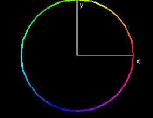
This demo shows a parametric curve in the x-y plane, with the different colors indicating different values of t. Try changing the functions x(t) and y(t) and the bounds and resolution for t.
|
Parametric Curves in Three-Space
| 
|
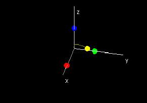
This demo includes five windows. The first window contains a slider bar allowing you to change the value of t. The next three windows show the graphs of (t, x(t)), (t, y(t)), and (t, z(t)). The last window shows the resulting parametric curve in three-space.
|
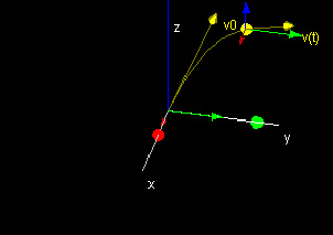
Example: Projectile Motion
| 
|
|
Exercises Parametrize the following curves:
- A line segment with endpoints (0, 0), (1, 0)
- A line segment with endpoints (2, 4, 7), (9, 8, 5)
- A circle of radius 1 centered on the origin in the x-y plane.
- A helix that starts at (1, 0, 0), ends at (1, 0, 10), has 10 loops, and contains points all of which are distance 1 from the z-axis.
In the second demo, add a new window containing a 2D graph that shows y as a function of x (do this by adding a curve whose parametrization is x(t), y(t) ). In the 3D graph window, select Up z-axis on the View menu. Try changing x(t), y(t), and z(t). How can you relate the 3D graph to the 2D graph you added? Why does this relationship exist?
|