« Course List

MA35 Labs

1 Single Variable Calculus

2 Two Variable Calculus

3 » Three Variable Calculus

Polar Coordinate Labs

Two Variable Functions

Contents

3.1 Functions of Three Variables

3.2 Differentiation

3.3 More Derivatives

3.4 Integration

3.5 Vector Analysis

3.5.1 Parametric Volumes

3.5.2 Path Integrals in Three-Space

3.5.3 Vector Fields, Curl and Divergence

3.5.4 Stokes' Theorem for Function Graphs

3.5.5 Conservative Vector Fields

3.5.6 Surface Integrals over Function Graphs

3.5.7 Gauss' Divergence Theorem for Regions between Function Graphs

Search

Stokes' Theorem for Function Graphs (Page: 1 | 2 )

Text

Stokes' Theorem states that for some vector field F and oriented surface S with boundary curve s,

∫∫_Scurl F ⋅ dS = ∫_s⁺F ⋅ ds.

Proof of Stokes Theorem:

At the beginning of the proof of Green's theorem, we examined a problem relating the value of some function P(x, y) at the point (x₀, c) to that value at the point (x₀, d). A more general problem is to find how the value of a function P(x, y, z) changes from a point (x₀, c, z(x₀, c)) to a point (x₀, d, z(x₀, d)), if we confine ourselves to the function graph of z(x, y).

If we travel a distance dy in the y direction, two events will occur. Firstly, there will be some change in P(x, y, z) due to the change in y, given by P_y(x, y, z)*dy. This occurrence is familiar to us from Green's theorem.

Secondly, since we are confining ourselves to the function graph of z(x, y), there must be some change dz in z as a result of the change in y, given by dz = z_y(x, y) * dy. This change in z causes a change in P(x, y, z) by the amount P_z(x, y, z) * dz = P_z(x, y, z) * z_y(x, y) * dy.

The net change in P(x, y, z) from y = c to y = d, then, is given by

P(x₀, d, z(x₀, d)) - P(x₀, c, z(x₀, c)) = ∫_c^d(P_y(x₀, y, z(x₀, y)) + P_z(x₀, y, z(x₀, y))*z_y(x₀, y))dy

By integrating the result above with respect to x from x = a to x = b, with c and d expressed as functions of x, we get a comparison between integrals over two different curves given by a double integral:

∫_a^bP(x, d(x), z(x, d(x)))dx - ∫_a^bP(x, c(x), z(x, c(x)))dx = ∫_a^b∫_c(x)^d(x)(P_y(x, y, z(x, y)) + P_z(x, y, z(x, y))*z_y(x, y))dydx

Now multiply by -1 and apply Fubini's theorem:

∫_a^bP(x, c(x), z(x, c(x)))dx - ∫_a^bP(x, d(x), z(x, d(x)))dx = ∫_a^b∫_c(x)^d(x)(-P_y(x, y, z(x, y)) + P_z(x, y, z(x, y))*-z_y(x, y))dxdy

If we wanted to include curves that connect (x, c(x), z(x, c(x))) to (x, c(x), z(x, c(x))) at x = a and x = b so that the left side of the equation above became a closed curve, this would be equivalent to adding 0, since x would not be changing along these curves. This allows us to write the following equation:

∫_s⁺P(x, y, z(x, y))dx = ∫∫_S(-P_y(x, y, z(x, y)) + P_z(x, y, z(x, y))*-z_y(x, y))dxdy

for some surface S (part of a function graph) and boundary s ("+" indicates that the direction of travel, projected onto the x-y plane, is counterclockwise when viewed from above). Let us refer to this result, for now, as part 1 of Stokes' Theorem for function graphs.

We can follow a similar process, switching the roles of x and y and considering some function Q(x, y, z) instead of P(x, y, z) to get "part 2":

∫_s⁺Q(x, y, z(x, y))dy = ∫∫_S(Q_x(x, y, z(x, y)) - Q_z(x, y, z(x, y))*-z_x(x, y))dxdy

"Part 3" is discussed on the next page.

Demos

Stokes' Theorem (Pdx term)

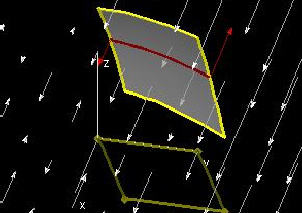
This demo verifies the statement P(x0, d, z(x0, d)) - P(x0, c, z(x0, c)) = ∫cd(Py(x0, y, z(x0, y)) + Pz(x0, y, z(x0, y))*zy(x0, y))dy made in the proof above (for y-simple domains), which is a crucial step in the proof of "part 1". The red arrows represent P(x, c, z(x, c)) and P(x, d, z(x, d)), the blue arrows represent Py(x0, y, z(x0, y))dy, and the green arrows represent Pz(x0, y, z(x0, y))*zy(x0, y))dy. In this demo as well as the next two, the white arrows represent whichever function of x, y, and z we are concerned with (P in this demo, Q in the next, and R in the last). The white lines in the "Changes in Pdx along the red curve" window serve two functions. The first is to show to which points on the curve the green and blue arrows correspond. The second use of these white lines is that the spacing between them indicates dy along the y-axis and dz along the z-axis. Note that the spacing is even for dy and uneven for dz. The vector sums window shows that the integral carried out over the red curve is equal to the difference between the lengths of the red arrows. You can change h to see that this is true throughout the given region, which allows us to integrate with respect to x and obtain "part 1". Try changing a, b, c(x), d(x), P(x, y, z), and z(x, y) as well.

Stokes' Theorem (Qdy term)

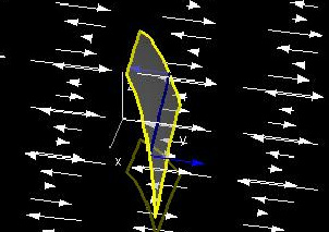
This demo is similar to the first, and verifies Q(b, y0, z(b, y0)) - Q(a, y0, z(a, y0)) = ∫ab(Qx(x, y0, z(x, y0)) + Qz(x, y0, z(x, y0))*zx(x, y0))dx for x-simple domains. This is one of the steps (not explicitly shown) which leads to "part 2". The blue arrows represent Q(a, y, z(a, y)) and Q(b, y, z(b, y)), the red arrows represent Qx(x, y0, z(x, y0))dx, and the green arrows represent Qz(x, y0, z(x, y0))*zx(x, y0))dx. As in the first lab, the white lines seen in the "Changes in Qdy along the blue curve" window show where on the curve the red and green arrows apply. The spacing between these lines represents the magnitudes of dx and dz. The vector sums window shows that the integral carried out over the blue curve is equals the difference between the lengths of the blue arrows. You can change h to see that this is true throughout the given region, which allows us to integrate with respect to y and obtain "part 2". Try changing a(y), b(y), c, d, Q(x, y, z), and z(x, y) as well.

Exercises