|
Stokes' Theorem for Function Graphs
(Page: 1
| 2 ) Text Proof of Stokes' Theorem (continued):

We have expressed the integrals of Pdx and Qdy over the boundary of some surface S as double integrals over S. Now suppose we want to consider the integral of some function R(x, y, z) with respect to z over the same boundary.
Let us first consider how this would work for the domain a≤x≤b, c≤y≤d.
Along the parts of the function graph of z(x, y) which lie above horizontal line segments (segments of the lines y = c and y = d), only x is changing. If we move along one of these curves a distance dx, the change dz in z is given by dz = zx(x, y)*dx.
We have found a way to express some integral with respect to z as an integral with respect to x. Specifically, rather than integrating R with respect to z over the boundary, we can integrate R*zx(x, y) with respect to x over the boundary.
To relate this integral to a double integral, first consider two points, one with y = c and one with y = d, which have the same x value, x0. The change in R*zx(x, y) from (x0, c, z(x0, c)) to (x0, d, z(x0, d)) is given by
R(x0, d, z(x0, d))*zx(x0, d) - R(x0, c, z(x0, c))*zx(x0, c) = ∫cd(∂(R(x0, y, z(x0, y))*zx(x0, y))/∂y)*dy
Use the product rule to evaluate the partial derivative on the right side of the equation:
R(x0, d, z(x0, d))*zx(x0, d) - R(x0, c, z(x0, c))*zx(x0, c) = ∫cd(R(x0, y, z(x0, y)))*zyx(x0, y)) + (Ry(x0, y, z(x0, y)))*zx(x0, y))*dy
Integrate this result with respect to x from x = a to x = b:
∫abR(x, d, z(x, d))*zx(x, d)*dx - ∫abR(x, c, z(x, c))*zx(x, c)*dx = ∫ab∫cd(R(x, y, z(x, y)))*zyx(x, y) + (Ry(x, y, z(x, y)))*zx(x, y)*dydx
Now multiply by -1 and apply Fubini's theorem:
∫abR(x, c, z(x, c))*zx(x, c)*dx - ∫abR(x, d, z(x, d))*zx(x, d)*dx = ∫ab∫cd-(R(x, y, z(x, y)))*zyx(x, y) + (Ry(x, y, z(x, y)))*-zx(x, y)*dxdy
If we apply a similar process to the parts of the function graph that lie above the segments of the lines x = a and x = b, we get the following result:
∫cdR(b, y, z(b, y))*zy(b, y)*dy - ∫cdR(a, y, z(a, y))*zy(a, y)*dy = ∫ab∫cd(R(x, y, z(x, y)))*zxy(x, y) - (Rx(x, y, z(x, y)))*-zy(x, y)*dxdy
If we add these last two equations together, there are two important observations that will simplify the result. The first is that the four integrals on the left side are equivalent to the integral of Rdz over the boundary for counterclockwise travel. The second is that, due to equality of mixed partials, two terms on the right side of the equation will cancel. The simplified result is:
∫s+R(x, y, z(x, y))dz = ∫∫S(Ry(x, y, z(x, y))*-zx(x, y) - Rx(x, y, z(x, y))*-zy(x, y))dxdy
Though we found this for a function graph that projects onto a rectangular domain, the result works for any domain D that is a simple region, since we can first look at the part of Rdz affected by changes in x, looking at D as a y-simple region, and can then look at the part of Rdz affected by changes in y, looking at D as an x-simple region. This proves "part 3" of Stokes' Theorem.
Now add together parts 1, 2, and 3 to get Stokes' Theorem:
∫s+P(x, y, z(x, y))dx + Q(x, y, z(x, y))dy + R(x, y, z(x, y))dz =
∫∫S([(Ry(x, y, z(x, y)) - Qx(x, y, z(x, y))]*-zx(x, y) + [Pz(x, y, z(x, y)) - Rx(x, y, z(x, y))]*-zy(x, y)) + [Qx - Py])dxdy
For a continuously differentiable vector field F = (P(x, y, z(x, y)), Q(x, y, z(x, y)), R(x, y, z(x, y))), this simplifies to
∫∫Scurl F ⋅ dS = ∫s+F ⋅ ds

Demos
Stokes' Theorem (Rdz term)
| 
|
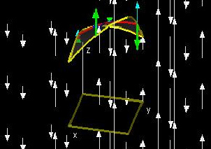
This demo tests "part 3" of Stokes' Theorem for rectangular domains of the form a≤x≤b, c≤y≤d. Specifically, it tests the statement
R(x0, d, z(x0, d))*zx(x0, d) - R(x0, c, z(x0, c))*zx(x0, c) = ∫cd(R(x0, y, z(x0, y)))*zyx(x0, y)) + (Ry(x0, y, z(x0, y)))*zx(x0, y))*dy
, which is evaluated along the red curve, and
R(b, y0, z(b, y0))*zy(b, y0) - R(a, y0, z(a, y0))*zy(a, y0) = ∫ab(R(x, y0, z(x, y0)))*zxy(x, y0)) + (Rx(x, y0, z(x, y0)))*zy(x, y0))*dy
, which is evaluated along the blue curve.
In the window showing the surface, the cyan arrows represent the value of R(x, y, z). The red and blue arrows represent zx(x, y) and zy(x, y), respectively. The green arrows at the endpoints of the red curve represent R(x, y, z)*zx(x, y), the product of the two other values represented at that endpoint. Similarly, the green arrows at the endpoints of the blue curve represent R(x, y, z)*zx(x, y).
The other two windows show how these values represented by the green arrows change as one moves along either the red or the blue curve across the surface. Each shows a graph of the values of R(x, y, z(x, y)) on one plane and a graph of either zx(x, y) or zy(x, y) on another plane, starting from one end of the respective curve on the function graph and going to the other end. The areas of the green rectangles correspond to the values of the products of the functions graphed in the planes (these products are R(x, y, z)*zx(x, y) and R(x, y, z)*zy(x, y)), and demonstrate the need for the product rule in the derivation of "part 3" of Stokes' Theorem.
You can change h and k to see how "part 3" works for different slices of the surface. Try changing a, b, c, d, R(x, y, z), and z(x, y) to test "part3" for different domains, expressions for R, and surfaces.
|
Exercises Describe what happens when you set z(x, y) equal to:
- 0
- Any constant
- Any linear function of x and y (ax + by + c)
Compare your results from Exercise 1 on this page to your results from Exercise 1 on the previous page.
|