Labware - MA35 Multivariable Calculus

Perhaps the most confusing aspect of Green's Theorem is that we are able to express information about a surface just by performing an integral over the boundary of the surface. Why is no information lost if we ignore the entire inner part of the surface?

We can relate the value of some function at one point on a boundary to that at another point on the boundary by adding up the changes in the value of that function as one travels across the surface from one point to the other. This allows us to relate function values on a boundary to partial derivatives of that function throughout the surface. Green's Theorem is one example of a relationship of this type that we can establish.

To see the derivation of Green's Theorem, please expand:

Let us first think about a simpler problem which will lead us to Green's Theorem.

Suppose we want to find out how the value of some function P(x, y) changes as we move from some point (x₀, c) to some point with a higher y value, (x₀, d). Part of the Fundamental Theorem of Calculus (∫_a^bf(x)dx = G(b) - G(a), where f(x) = G'(x)) gives us the information we want:

∫_c^dP_y(x,y)dy = P(x₀, d) - P(x₀, c).

Now suppose that we have two functions, c(x) and d(x) (with d(x) > c(x)), and we want to compare the values of P for each set of points c(x) and d(x) that have the same x value, over some domain a≤x≤b. Essentially, we can integrate our result from above with respect to x from x = a to x = b to get the desired result. (Note that the double integral will be carried out over the region between c(x) and d(x), since we are considering the set of all line segments joining points in c(x) to points in d(x)):

∫_a^b∫_c(x)^d(x)P_y(x,y)dydx = ∫_a^bP(x, d(x))dx - ∫_a^bP(x, c(x))dx.

Now multiply by -1:

-∫_a^b∫_c(x)^d(x)P_y(x,y)dydx = ∫_a^bP(x, c(x))dx - ∫_a^bP(x, d(x))dx.

The integral of anything with respect to x for vertical line segment paths is 0 since x doesn't change along those paths, so we can add in two terms on the right side of the equation to complete a curve around which one is traveling counterclockwise (i.e. + sign for lower curve, c(x), and - sign for upper curve, d(x)). Our result is lemma 1 of Green's theorem:

∫_C⁺P(x, y)dx = -∫∫_DP_y(x, y)dxdy for a function P(x,y) and a y-simple region D with boundary C ("+" indicates counterclockwise travel). Note that Fubini's theorem allowed us to change the order of integration.

We can find lemma 2 of Green's theorem using almost the same process, with the roles of x and y switched. The main difference relates to direction of travel. For lemma 1, we had d(x) > c(x), and counterclockwise travel meant increasing x on the lower-valued curve,c(x), and decreasing x on the higher-valued curve, d(x). For lemma 2, counterclockwise travel causes us to increase y for the higher-valued curve, b(y), and decrease y for the lower-valued curve, a(y). The result is

∫_C⁺Q(x, y)dy = ∫∫_DQ_y(x, y)dxdy. This time D must be an x-simple region.

We know that for a simple region, both lemmas will be true, so we can add them to get Green's theorem:

∫_C P(x,y) dx + Q(x,y) dy = ∫∫_D (- P_y(x, y) +Q_x(x, y)) dxdy.

The proof of Green's theorem for non-simple regions is left as an exercise.

Demos

Green's Theorem: Lemma 1

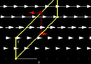
In this demonstration of the first lemma used in Green's Theorem, the two dark red points joined by the line segment are the points we considered at the beginning of the discussion above.
The vector field shows the values of P(x, y) (right = positive, left = negative).
The lower and higher bright red vectors correspond to the value of P(x, c(x)) and the value of -P(x, d(x)), respectively.
Finally, the dark red vectors correspond to the values of -P_y(x, y). Their sum represents the integral which is equal to the sum of the bright red vectors, as shown in the "Vector Sums" window. This corresponds to the equation ∫_c^dP_y(x,y)dy = P(x₀, d) - P(x₀, c). You can change h (the x value of the vertical line segment) to see that this equation is true for the whole region.
You can change the region by changing a, b, c(x), and d(x), and you can also change the expression for P(x,y).

Green's Theorem: Lemma 2

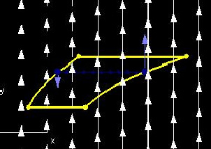
In this lemma 2 demo, vector field shows the values of Q(x, y) (up = positive, down = negative).
The light blue vectors, one on the curve (y(a), y), and the other to its right on the curve (y(b), y), correspond to the value of -Q(a(y), y) and the value of Q(b(y), b), respectively.
Finally, the dark blue vectors correspond to the values of Q_x(x, y). The sum of the light blue vectors equals the sum of the dark blue vectors, corresponding to the equation ∫_a^bQ_x(x,y)dx = Q(x₀,b)-Q(x₀,a).
This time, you can change k (the y value of the vertical line segment) to see that this equation is true for the whole region.
You can change the region by changing a(y), b(y), c, and d, and you can also change the expression for Q(x,y).

Examples

Circular Region (Lemma 1)

a = -1

b = 1

c(x) = √(1 - x²)

d(x) = -√(1 - x²)

Increase resolution of x to 20 or higher.

Circular Region (Lemma 2)

a(y) = √(1 - x²)

b(y) = -√(1 - x²)

c = -1

d = 1

Increase resolution of y to 20 or higher.

Exercises

1. In the Lemma 1 demo, try this example:

P(x, y) = y²

a = 0

b = 2

c(x) = x²

d(x) = x + 2

What happens in the Vector Sums window when h is equal to b, its maximum value? Why does this occur?

2. How does the "Vector Sums" window in each of these demos show how Green's theorem relates to the Fundamental Theorem of Calculus?

3. Why can you construct any right triangle with legs parallel to the axes for both of these demos? How can you use this to prove Green's theorem for non-simple regions?

4. How do the methods used in these demos show that Green's theorem only works for closed regions?